Sensitivity Analysis in Real Estate: Stress-Testing a Deal
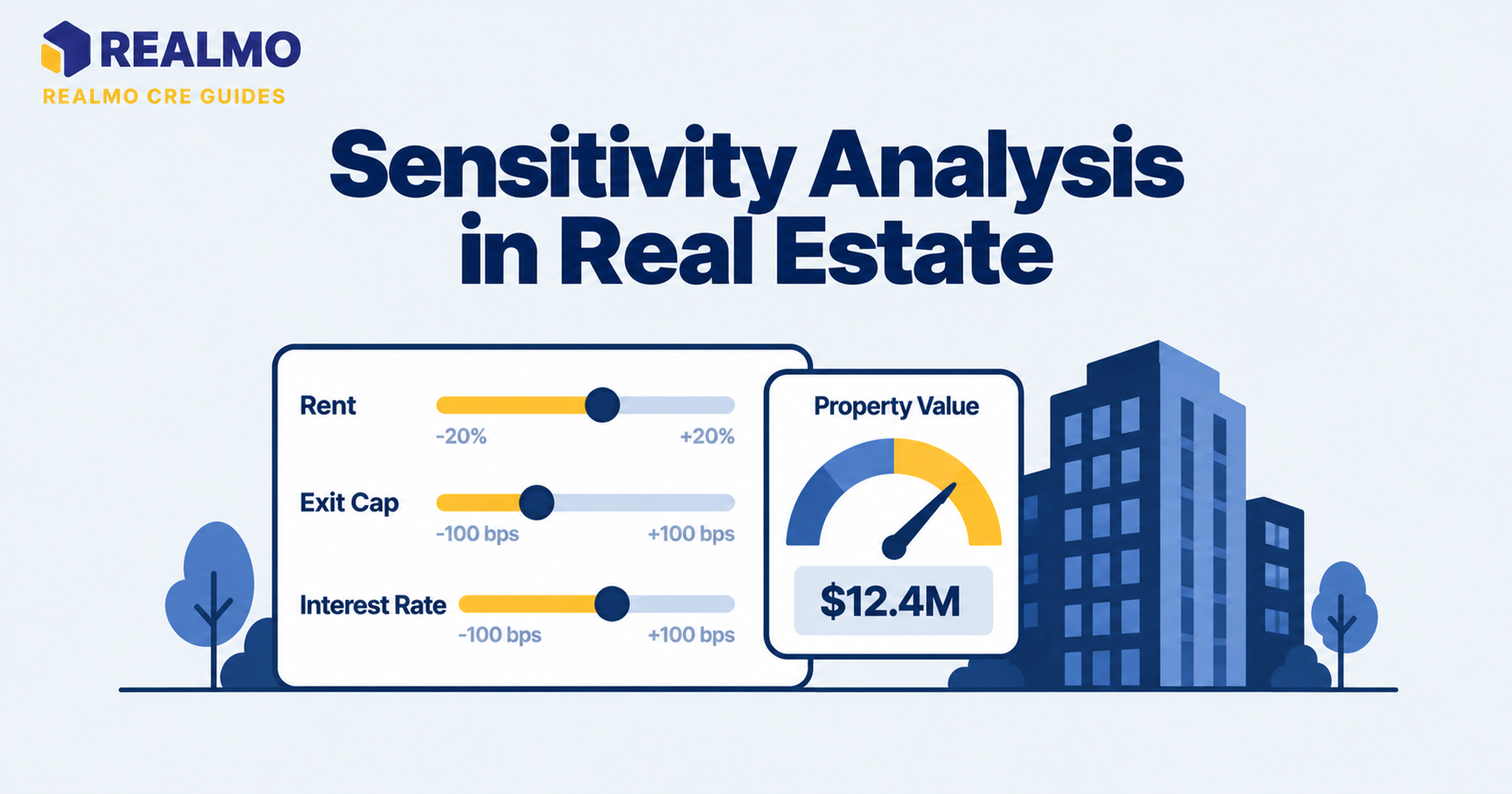
Sensitivity analysis in real estate is the practice of changing one or two underwriting assumptions at a time and recording what happens to returns. It answers a narrow question: which inputs actually decide whether this deal works, and how far can they move before it doesn’t.
Why a base case alone is not underwriting
An investor models a value-add flex building, lands on a 15% levered IRR, and takes that number to the investment committee. The committee asks what happens if the exit cap comes in fifty basis points wider than going-in. The investor doesn’t know, because the model produced one answer to one set of guesses.
That single number carries false precision. Every input in it , rent growth, downtime between tenants, renovation cost, refinance proceeds, exit pricing , was an estimate made months before the outcome. Sensitivity analysis converts the model from a prediction into a map of outcomes. It tells the investor that the deal survives a 100-basis-point exit cap expansion but breaks if lease-up takes nine months instead of four. That is a usable finding: it points at where diligence dollars and contract protections should go.
What sensitivity analysis in real estate measures
The method isolates cause and effect. Hold every input fixed, move one, and the change in internal rate of return or equity multiple is attributable to that input alone. Do this across several variables and they sort themselves into a rough hierarchy, the ones that swing the outcome, and the ones that barely register.
That hierarchy is the actual product. Underwriting time is finite, and a sensitivity table shows where it belongs. If a 20% miss on the property management fee moves IRR by twenty basis points, stop arguing about the management fee. If a half-point of exit cap moves it three hundred, the exit assumption deserves comparable sales work, not a round number.
Sensitivity analysis is distinct from scenario analysis. This moves several correlated inputs together into a coherent story, a recession case where rent growth falls, vacancy rises, and cap rates widen at once. Sensitivity isolates; scenarios combine. Serious underwriting uses both, and Monte Carlo simulation extends the idea further by sampling thousands of input combinations from probability distributions.
Which inputs move returns and which are noise
In most deals, four inputs dominate. Exit capitalization rate is usually first, because it prices the largest single cash flow in the model and is the assumption made furthest from any observable evidence. Timing runs a close second , lease-up speed, renovation delivery, hold period , because IRR is time-weighted and a delayed dollar is a smaller dollar. Rent achieved on turnover is third, since it compounds through the hold and feeds the exit value. Financing terms come fourth: rate, proceeds, and amortization set the size and shape of levered cash flow.
Inputs that do not move the needle include small line items in the operating expense stack. Modest changes in the reserve figure, and marginal shifts in transaction costs. They still belong in the model for accuracy, but they don’t belong in the sensitivity grid.
The ranking shifts by property type. In single-tenant net lease, credit and rollover risk sit almost entirely at the lease expiration date, so hold period and renewal probability dominate. In multi-tenant office, releasing cost and downtime per rollover matter more than headline rent. In hospitality, where revenue reprices nightly, operating margin sensitivity outweighs almost everything else.
One-way tables versus two-way grids
A one-way table moves a single variable across a range and reports one output. It is the right tool for ranking inputs against each other, because each result is clean.
A two-way grid crosses two variables and shows their joint effect. It is the right tool once the two dominant inputs are identified, since it reveals whether a bad outcome on one can be absorbed by a good outcome on the other. Its risk is implying that the two axes are independent when they usually are not , cap rates and rent growth both respond to the same economic conditions, and a grid cell showing weak rent growth alongside cap rate compression may describe a state of the world that rarely occurs.
How to set an honest range for each variable
The range determines the finding, which makes it the most manipulable part of the exercise. A narrow band around a favorable base case produces a table where nothing bad happens.
Anchor ranges in observable history rather than comfort. For exit cap rates, look at where the asset type traded across a full cycle in that market. This includes the widest points, and use spread relationships rather than a single remembered figure. For construction cost, ask the general contractor what the last three comparable projects ran over budget by. For lease-up, find how long competing space in the submarket actually sat before signing.
Ranges should be asymmetric when reality is asymmetric. Renovation budgets overrun more frequently than they underrun, and lease-up runs late more frequently than early. A symmetric plus-or-minus band on those inputs quietly flatters the deal. Pulling ownership records, prior sale pricing, and comparable valuations , the kind of data available across Realmo’s property analytics , gives the range a defensible starting point instead of a guess.
Worked example: a two-way equity multiple grid
All figures below are illustrative and rounded for clarity.
Assume a $10,000,000 acquisition at $650,000 of Year 1 net operating income. The loan is $6,000,000 interest-only at 6%, with $360,000 annual debt service. Equity is $4,000,000. The hold is five years, selling costs are 2%, and exit pricing uses forward-year NOI. The base case assumes 3% annual NOI growth and a 6.5% exit cap.
Base case mechanics: Year 6 NOI is $650,000 × 1.03⁵ = $753,528. At a 6.5% exit cap, gross value is $11,592,700; net of 2% costs and loan repayment, sale proceeds are $5,360,846. Five years of operating cash flow after debt service total $1,650,939. Distributions of $7,011,785 on $4,000,000 of equity produce a 1.75x equity multiple.
Crossing NOI growth against exit cap:
| NOI growth ↓ / Exit cap → | 6.0% | 6.5% | 7.0% |
|---|---|---|---|
| 1% | 1.67x | 1.45x | 1.27x |
| 3% | 1.99x | 1.75x | 1.55x |
| 5% | 2.34x | 2.07x | 1.85x |
Interpretation: the deal returns capital plus a margin in every cell, so the downside question is not loss of principal but whether the worst corner clears the investor’s required return. The grid appears to show growth mattering more than exit pricing , a 1.45x-to-2.07x swing on the growth axis against 1.99x-to-1.55x on the cap axis. That comparison is an artifact of the ranges chosen: growth was given a ±2-point band and the cap a ±0.5-point band. Per unit of plausible movement, the exit cap is the harder input.
Common error: reading the grid as a probability distribution. It shows what happens in each cell, not how likely each cell is.
Where sensitivity tables stop being useful
A table cannot capture non-linear events. Tenant default, a lender declining to extend, an insurance market repricing coastal risk , these are step changes, not gradual shifts along an axis, and they belong in scenario work.
Sensitivity also assumes the model structure is correct. If the pro forma omits a capital item or misdates a lease expiration, every cell in the grid is wrong by the same amount. Stress-testing tests assumptions, not arithmetic. Model review comes first.
Common mistakes when stress-testing a deal
- Ranging around the base case instead of around history. The output looks resilient because the inputs were never allowed to reach realistic bad values, and the committee approves a deal that was never actually tested.
- Flexing revenue without flexing timing. Slower absorption changes both the amount and the arrival date of cash flow; testing rent alone understates the IRR impact of a soft market.
- Leaving debt static. If exit cap rates widen, the refinance assumption embedded in Year 3 probably shouldn’t hold either, and a deal that clears the equity test can still fail a debt service coverage test.
- Testing eight variables and acting on none. A wall of tables with no ranking produces no decision. The point is to identify the two or three inputs worth negotiating protection against.
- Treating the worst cell as the floor. Correlated inputs can move together beyond the grid’s corners; the table’s edge is where the analysis stopped, not where risk stopped.
Related terms
Internal Rate of Return (IRR) · Net Operating Income (NOI) · Exit Cap Rate · Equity Multiple · Debt Service Coverage Ratio · Discounted Cash Flow Analysis · Pro Forma · Break-Even Occupancy
FAQ
What is sensitivity analysis in real estate underwriting?
It is the process of varying one or two model inputs across a defined range while holding the rest constant, then recording how returns respond. The output is a table showing which assumptions control the outcome and how much room the deal has before returns fall below the investor’s threshold.
How is sensitivity analysis different from scenario analysis?
Sensitivity isolates a single variable to measure its individual effect. Scenario analysis moves multiple correlated variables together to describe a plausible state of the world. Examples include a downturn with slower rent growth, higher vacancy, and wider cap rates. Sensitivity ranks inputs; scenarios test coherent narratives.
Which variables should be stress-tested first?
Start with exit cap rate, timing assumptions such as lease-up and hold period, achievable rent on rollover, and financing terms. These four account for most of the return variance in a value-add deal. Small operating expense lines rarely justify a place in the grid.
How wide should sensitivity ranges be?
Wide enough to include values the market has actually produced across a full cycle, not a narrow band around the base case. Ranges should be asymmetric where outcomes are asymmetric, renovation budgets and lease-up periods overrun more than they come in early.
Does sensitivity analysis predict returns?
No. It maps how the model responds to changed inputs and assigns no probability to any cell. A grid showing a 1.27x downside case says what happens at those inputs, not how likely those inputs are.