CRE Return Metrics: IRR, Cash-on-Cash and Equity Multiple
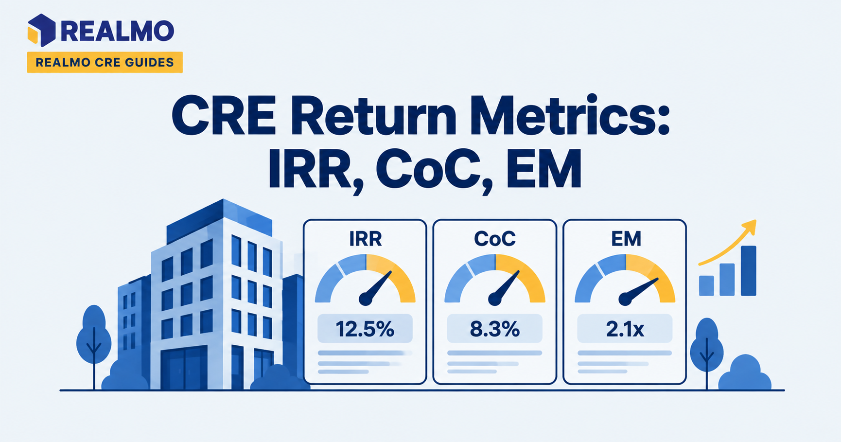
Commercial real estate returns are measured with three complementary metrics: cash-on-cash return, which tracks annual pre-tax cash flow against equity invested. Equity multiple, which shows total dollars returned per dollar contributed; and internal rate of return (IRR), which weights every dollar by when it arrives. Each answers a different question, and no single one is sufficient.
Why the three metrics rarely agree
Picture two deals on your desk. A stabilized single-tenant industrial building projects a 7% cash-on-cash return in year one, a 1.6x equity multiple, and a 12% IRR over seven years. A value-add multi-tenant flex property projects negative cash flow for eighteen months, a 1.9x equity multiple, and an 18% IRR over four years. The second deal wins on IRR and multiple. The first wins on distributions you can actually spend.
Neither answer is wrong, because the metrics measure different things. Choosing between the deals requires knowing which constraint binds you: current income, total wealth accumulated, or speed of capital recycling. Investors who look only at IRR systematically overweight short holds with aggressive exit assumptions. Investors who look only at cash-on-cash systematically underweight appreciation and repayment of principal. The discipline is reading all three together and knowing what each one hides.
How commercial real estate returns are measured
Every return metric starts from the same chain of cash: gross potential rent, less vacancy and credit loss, less operating expenses, produces net operating income. NOI less debt service produces cash flow before tax. Cash flow before tax, less capital expenditures funded from operations and plus or minus reserve activity, produces the distributable cash an equity investor actually receives.
Return metrics diverge based on where in that chain they measure and whether they account for the passage of time. Cash-on-cash and IRR are usually calculated after debt service, they describe what the equity earns. Cap rate sits above the debt line entirely and describes the asset, not the investor. Confusing the two levels is the single most common source of miscommunication between sponsors and passive investors.
A second distinction runs through all three metrics: pre-tax versus after-tax. Standard practice in offering materials is pre-tax, because depreciation schedules, passive activity limits, and the investor’s own bracket are outside the sponsor’s control. An investor comparing a leveraged real estate deal to a taxable bond is not comparing like with like unless both sides are adjusted. Consult a licensed tax professional before drawing conclusions about after-tax outcomes in your own situation.
Cash-on-cash return: annual yield on equity
Cash-on-cash return divides one year’s pre-tax cash flow by the total equity invested to date. It answers a narrow, useful question: what percentage of my money came back to me this year, in cash?
Cash-on-Cash Return = Annual Pre-Tax Cash Flow ÷ Total Equity Invested
Total equity invested is not the down payment alone. It includes closing costs, loan fees, due diligence expense, upfront capital reserves, and any acquisition fee paid to a sponsor. Understating the denominator inflates the metric, and it is a frequent source of quiet overstatement in marketing materials.
Using illustrative round numbers: an investor contributes $1,500,000 in total equity and receives $120,000 of distributions in year three. Cash-on-cash return for that year is $120,000 ÷ $1,500,000 = 8.0%. If year four distributions rise to $135,000 on the same equity base, year four cash-on-cash is 9.0%.
Because the metric is annual and unweighted, it produces a different number every year of the hold. Sponsors quoting a single figure are usually citing either year one, the average across the hold, or the stabilized year, three materially different claims. Ask which. The average across a hold with an eighteen-month lease-up will look nothing like year one.
Cash-on-cash return also ignores principal amortization, which builds equity without touching the distribution line, and ignores the sale entirely. A deal can post a modest cash-on-cash return every year and still deliver most of its profit at exit. That gap is what the other two metrics exist to close.
Equity multiple: total dollars back per dollar in
Equity multiple divides all distributions received, including sale proceeds, by all equity contributed. It is expressed as a multiple rather than a percentage, and it ignores timing completely.
Equity Multiple = Total Distributions ÷ Total Equity Invested
A 1.0x multiple means the investor got their money back and nothing more. A 2.0x multiple means the investment doubled. Anything below 1.0x is a loss of principal, regardless of how strong the annual cash-on-cash looked along the way.
The metric’s virtue is that it cannot be manipulated by shortening the hold. Its weakness is the mirror image: it treats a dollar returned in year one identically to a dollar returned in year ten. A 2.0x over five years and a 2.0x over twelve years are the same number and are not remotely the same investment.
Equity multiple is the right lens when the question is total wealth created rather than speed. It is also the metric that survives contact with reality best. This is because it depends on actual dollars in and out rather than on a discount rate calculation that can be reshaped by assumption changes.
IRR: the return metric that prices time
IRR is the discount rate at which the present value of all cash flows, including the initial equity outlay, equals zero. In plain terms, it is the annualized rate of return the investment earns on capital while that capital remains at risk.
IRR has no closed-form solution for a typical deal; it is solved iteratively, which is why spreadsheets use IRR and XIRR functions rather than a formula you can compute by hand. XIRR is the more accurate choice for real deals because it uses actual dates rather than assuming even periods , quarterly distributions and a mid-month closing are not annual events.
Two properties of IRR drive most of the confusion around it. First, IRR rewards early cash. A refinance in year two that returns half the equity will lift IRR substantially even if total distributions never change. This is because capital that comes home early stops being discounted. Second, IRR implicitly assumes distributions are reinvested at the IRR itself. For a deal projecting a high IRR, that assumption is usually unrealistic. This is why modified IRR (MIRR) exists and why sophisticated investors treat very high projected IRRs with more suspicion than enthusiasm.
IRR is also acutely sensitive to the exit assumption. In a typical five-to-seven-year hold on a stabilized asset, the majority of the projected return arrives at sale, and the sale price is a function of the exit cap rate applied to a forecast NOI. Shift that cap rate assumption modestly and the IRR moves substantially. Any IRR presented without the exit assumption stated next to it is an incomplete number.
Why IRR and equity multiple pull apart
The tension between these two metrics is structural, not a modeling error. IRR is time-weighted; equity multiple is not. Shorten the hold and IRR rises while the multiple stays flat or falls. Extend the hold and the multiple grows while IRR decays.
Consider a clean illustration with no interim cash flow. An investment that doubles equity over five years produces an IRR of roughly 14.9%. The same doubling stretched to eight years produces roughly 9.1%. Identical multiple, dramatically different annualized return, because the second version tied up capital for three additional years to accomplish the same thing.
Read together, the pair tells you something neither tells alone. High IRR with a low multiple signals a fast flip: capital comes back quickly but the absolute profit is thin, and the investor immediately faces reinvestment risk with no guarantee the next deal is as good. High multiple with a modest IRR signals a long hold with real wealth creation but slow capital turnover, frequently financed by amortization and rent growth rather than by a repositioning event.
This is also where fee structures matter. A sponsor whose promote is triggered by an IRR hurdle has an incentive toward shorter holds and earlier refinances. A sponsor compensated on the multiple has the opposite tilt. Reading the equity waterfall alongside the return projections tells you which behavior the deal is engineered to produce.
Levered vs. unlevered returns and what debt hides
Unlevered returns treat the property as if purchased for cash. Levered returns account for the loan. The gap between them is the contribution of financing, and it runs in both directions.
When the cost of debt is below the property’s unlevered yield, borrowing lifts equity returns, positive leverage. When the cost of debt exceeds the unlevered yield, borrowing drags equity returns down, negative leverage. Even though the deal may still pencil on a total-return basis because of amortization and appreciation. The sign of that relationship changes as rates move. This is why an identical property underwritten in two different financing environments produces different levered IRRs from the same NOI.
Debt also amplifies dispersion. Higher loan-to-value raises projected equity returns in the base case and raises the probability of total equity loss in the downside case. Two deals showing the same levered IRR can carry entirely different risk profiles if one is modestly financed and the other is stretched. The unlevered IRR strips financing out and lets you compare the assets themselves. The debt service coverage ratio tells you how much NOI decline the capital stack can absorb before the loan is in trouble.
The practical discipline: look at unlevered IRR to judge the real estate, levered IRR to judge your equity position, and DSCR to judge whether the structure survives a bad year.
What these metrics still don’t tell you
None of the three says anything about risk. A 20% projected IRR on a ground-up development in a thin submarket and a 20% projected IRR on a stabilized asset with an investment-grade tenant are the same number attached to entirely different probability distributions. Return metrics describe the base case; they are silent on the range of outcomes around it.
They are also silent on liquidity. Real estate equity is in prevailing market practice not redeemable on demand, and a projected exit year is a plan rather than a commitment. Sale timing is subject to market conditions, loan prepayment terms, and partner consent, and a hold extended by two years past plan compresses IRR whether or not the property performed.
Finally, all three are pre-tax by convention and ignore depreciation entirely. This means they systematically understate the after-tax result for many investors while ignoring depreciation recapture at sale. They also assume the capital expenditures reserve was sized correctly. A model that underfunds roof replacement and tenant improvements produces excellent metrics and an unpleasant year four.
Worked example: a five-year hold from entry to exit
All figures below are illustrative round numbers chosen to make the arithmetic legible, not market projections.
An investor acquires a multi-tenant property for $5,000,000 with a $3,500,000 loan. Total equity invested, including closing costs and upfront reserves, is $1,500,000.
Step 1, Lay out the cash flows. Distributions after debt service run $90,000 in year one, $105,000 in year two. $120,000 in year three, $135,000 in year four, and $150,000 in year five as lease-up completes and rents step up. Net sale proceeds at the end of year five, after loan payoff and transaction costs, are $2,400,000.
Step 2, Calculate cash-on-cash. Year one is $90,000 ÷ $1,500,000 = 6.0%. Year five is $150,000 ÷ $1,500,000 = 10.0%. Total operating distributions across the hold are $600,000, so the average annual cash-on-cash is $600,000 ÷ 5 ÷ $1,500,000 = 8.0%.
Step 3, Calculate equity multiple. Total distributions are $600,000 of operating cash plus $2,400,000 at sale = $3,000,000. Equity multiple is $3,000,000 ÷ $1,500,000 = 2.00x. Total profit is $1,500,000.
Step 4 , Calculate IRR. The cash flow series is −$1,500,000 at time zero, then $90,000, $105,000, $120,000, $135,000, and $2,550,000 (year five distributions plus sale proceeds). Solving for the rate that sets net present value to zero gives an IRR of approximately 16.4%.
How to interpret the three numbers. The 8.0% average cash-on-cash is what the investor could spend along the way. The 2.00x says the investment doubled. The 16.4% IRR says the doubling happened fast enough to beat a plain five-year doubling (14.9%), because interim distributions returned capital before the sale. Note also that roughly 80% of total dollars returned arrive in a single event , the exit. That concentration is the deal’s real risk, and it is invisible in any of the three headline metrics.
The common error here. Investors frequently compare that 16.4% IRR against the 6.0% year-one cash-on-cash and conclude the property “yields 16.4%.” It does not. The IRR includes $2,400,000 of sale proceeds that depend on a forecast NOI, a forecast exit cap rate, and a market that permits a sale in year five. Change the exit assumption and the IRR moves; the year-one cash-on-cash does not move at all. Underwriting entry and exit assumptions against actual valuation, ownership, and comparable-sale data , the kind of property-level analytics available across Realmo’s listing and property database , is what separates a defensible exit number from a hopeful one.
Common mistakes when reading return projections
- Quoting an IRR without stating the exit cap rate and hold period. The number becomes uninterpretable. Two sponsors can present the same property with IRRs several hundred basis points apart purely through exit assumptions, and the investor has no way to compare unless the assumption is disclosed.
- Understating total equity in the cash-on-cash denominator. Excluding closing costs, loan fees, and upfront reserves inflates every year’s cash-on-cash. On a deal where those items represent a meaningful share of capital in. The reported return can be overstated by a full percentage point or more.
- Treating average cash-on-cash as year-one income. An investor budgeting distributions against the average will be short in the early years of any lease-up or repositioning deal. Sometimes for the entire first half of the hold. This is a real cash-planning failure, not a modeling nuance.
- Comparing a levered IRR to an unlevered IRR. The comparison is meaningless, and it consistently makes the leveraged deal look superior on return while concealing that it also carries the entire risk of the debt.
- Ignoring the waterfall. Deal-level IRR and investor-level IRR differ by the sponsor’s promote. A projection showing an 18% deal-level IRR may deliver materially less to the limited partner after the promote tiers clear, and the two figures are frequently presented without labels.
- Assuming the hold period is fixed. Extensions past the projected exit compress IRR mechanically. A five-year plan that becomes a seven-year hold at the same sale price loses several points of annualized return without anything having gone wrong operationally.
Related terms
- Net operating income (NOI)
- Cap rate
- Debt service coverage ratio (DSCR)
- Exit cap rate
- Equity waterfall and preferred return
- Loan-to-value (LTV)
- Capital expenditures and reserves
- Cash flow after debt service
FAQ
Which return metric matters most in commercial real estate?
None of them individually. Cash-on-cash governs whether the investment funds current spending needs, equity multiple governs total wealth created, and IRR governs how efficiently capital was used over time. Institutional underwriting looks at all three plus downside sensitivities. An investor with income needs weights cash-on-cash more heavily; an investor compounding capital weights IRR and multiple.
Is a higher IRR always better?
No. IRR rises when hold periods shorten, so a shorter, thinner deal can post a higher IRR than a longer deal that creates more total profit. IRR is also highly sensitive to exit assumptions and implicitly assumes distributions are reinvested at the same rate. Always read IRR next to the equity multiple, the hold period, and the stated exit cap rate.
What’s the difference between cash-on-cash return and cap rate?
Cap rate divides NOI by property value and describes the asset before any financing. Cash-on-cash divides after-debt-service cash flow by equity invested and describes the investor’s position. The same property produces one cap rate and as many cash-on-cash returns as there are possible capital structures.
Why does my equity multiple look good while my IRR looks weak?
That pattern usually means a long hold. Equity multiple ignores time entirely, so a slow doubling and a fast doubling report identically, while IRR penalizes the slow one. It can also indicate that most profit arrives at sale rather than through interim distributions, which delays capital return and depresses the annualized figure.
Should IRR be calculated before or after tax?
Sponsor projections are conventionally pre-tax, because depreciation benefits, passive activity limitations, and marginal rates vary by investor. After-tax IRR is the more relevant figure for a personal decision but requires assumptions specific to your circumstances. A licensed tax advisor should run that analysis before it informs an investment decision.